This article is a continuation of my series of articles on Model Interpretability and Explainable Artificial Intelligence. If you haven’t read the first two articles, I highly recommend doing so first.
The first article of the series, ‘Introduction to Machine Learning Model Interpretation’, covers the basics of Model Interpretation. The second article, ‘Hands-on Global Model Interpretation’, goes over the details of global model interpretation and how to apply it to a real-world problem using Python.
This article picks up where we left off by diving into local model interpretation. First, we will look at what local model interpretation is and what it can be used for. Then we will dive into the theory of two of its most popular methods, Lime (Local Interpretable Model-Agnostic Explanations) and Shapley Value, and apply them to get information about individual predictions on the heart disease dataset.
What is local model interpretation?
Local model interpretation is a set of techniques aimed at answering questions like:
- Why did the model make this specific prediction?
- What effect did this specific feature value have on the prediction?
Using our domain expertise combined with the knowledge gained using local model interpretation, we can make decisions about our model, like if it is suitable for our problem or if it is not functioning as it’s supposed to.
The use of local model interpretation is getting increasingly important these days because a company (or individual) must be able to explain the decisions of their model, especially if it is getting used in a domain that requires a lot of trust, like for medicine or finances.
LIME (Local Interpretable Model-Agnostic Explanations)
Despite widespread adoption, machine learning models remain mostly black boxes. Understanding the reasons behind predictions is, however, quite important in assessing trust, which is fundamental if one plans to take action based on a prediction, or when choosing whether to deploy a new model. — Ribeiro, Marco Tulio, Sameer Singh, and Carlos Guestrin. “Why should I trust you?”
Concept and Theory
Lime, Local Interpretable Model-Agnostic, is a local model interpretation technique using Local surrogate models to approximate the predictions of the underlying black-box model.
Local surrogate models are interpretable models like Linear Regression or Decision Trees that are used to explain individual predictions of a black-box model.
Lime trains a surrogate model by generating a new dataset from the data point of interest. The way it generates the dataset varies dependent on the type of data. Currently, Lime supports text, image, and tabular data.
For text and image data, LIME generates the dataset by randomly turning single words or pixels on or off. In the case of tabular data, LIME creates new samples by permuting each feature individually.
The model learned by LIME should be a good local approximation of the black-box model, but that doesn’t mean that it’s a good global approximation.
Advantages
LIME is a good pick for analyzing predictions because it can be used for any black-box model, no matter if it is a deep neural network or an SVM. Furthermore, LIME is one of the only interpretation techniques that works for tabular, text, and image data.
Disadvantages
The definition of the neighborhood of the data-point of interest is very vague, which is a huge problem because that means that you have to try different kernel settings for most applications.
Furthermore, the explanations can be unstable, meaning that the explanation of two very close data-points can vary greatly.
For more information on LIME and Explainable AI, in general, check out Christoph Molnar’s excellent book “Interpretable Machine Learning”.
Example and Interpretation
LIME can be used in Python with the Lime and Skater packages, making it really easy to use LIME with models from popular machine learning libraries like Scikit Learn or XGBoost. For this article, I’ll work on the Heart Disease dataset, a simple classification dataset.
To analyze the predictions of a tabular dataset like the Heart Disease dataset, we need to create a LimeTabularExplainer.
import lime
import lime.lime_tabular

rf = RandomForestClassifier().fit(X_train, y_train)
explainer = lime.lime_tabular.LimeTabularExplainer(np.array(X_train), feature_names=df.drop(['target'], axis=1).columns.values, class_names=rf.classes_, discretize_continuous=True)
Now we can use the explain_instance method to explain a single prediction.
exp = explainer.explain_instance(X_test.iloc[0], rf.predict_proba)
exp.show_in_notebook(show_table=True, show_all=False)
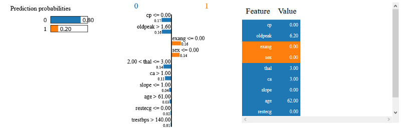
Here we can nicely see what feature values influenced the prediction. For this data-point, the cp and oldpeak values had the most negative influence on the prediction.
For more examples of using Lime, check out the “Tutorials and API” section in the README file.
Shapley Values
The Shapley value is a method for assigning payouts to players depending on their contribution to the total payout. But what does this have to do with Machine Learning?
Overview
In the case of machine learning, the “game” is the prediction task for a data point. The “gain” is the prediction minus the average prediction of all instances, and the “players” are the feature values of the data point.
The Shapley value is the average marginal contribution of a feature value across all possible coalitions. It is an excellent way of interpreting an individual prediction because it doesn’t only give us the contribution of each feature value, but the scale of these contributions is also correct, which isn’t the case for other techniques like LIME.
To get more information about Shapley Values and how they are calculated, be sure to check out the Shapley Values section of Christoph Molnar’s book “Interpretable Machine Learning”.
Advantages
When using Shapley values, the prediction and the average prediction are fairly distributed among the feature values of the instance. This makes Shapley Values perfect for situations that need an exact explanation. Furthermore, Shapley value is the only local explanation method with solid theory behind it.
Disadvantages
The Shapley value requires a lot of computing time. Most often, only the approximate solution is feasible. Another disadvantage is that you need access to the data to calculate the Shapley value. This is because you need the data to replace parts of the instance of interest. This problem can only be avoided if you can create data instances that look like real data instances.
Example and Interpretation
We can use Shapley values in Python using the excellent shap (SHapley Additive exPlanations) package created by Scott Lundberg.
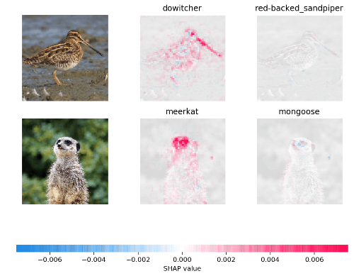
The shap package can be used for multiple kinds of models like trees or deep neural networks as well as different kinds of data, including tabular data and image data.
To use shap with the heart disease dataset, we can create a TreeExplainer that can explain the predictions of tree models like a Random Forest and then use the shap_values and force_plot methods to analyze predictions.
import shap
shap.initjs()
model_lgb = lgb.LGBMClassifier().fit(X_train, y_train)
# Create a object that can calculate shap values
explainer = shap.TreeExplainer(model_lgb)
# Calculate Shap values
shap_values = explainer.shap_values(np.array(X_test))
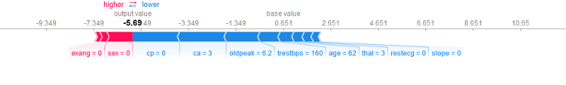
shap.force_plot(explainer.expected_value, shap_values[0,:], X_test.iloc[0,:])
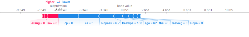
In the image, we can see how each feature value affects the prediction. In this case, the predicted value is 0, which means the patient doesn’t have heart disease. The most significant feature values are cp=0 and ca=3. This is indicated by the length of the arrows.
Conclusion
Local model interpretation is a set of techniques trying to help us understand individual predictions of machine learning models. LIME and Shapley value are two techniques to understand individual predictions.
Lime is very good for getting a quick look at what the model is doing but has problems with consistency. On the other hand, Shapley value delivers a full explanation, making it a lot more exact than Lime.
That’s all from this article. If you have any questions or want to chat with me, feel free to contact me via EMAIL or social media.