Hands-on Global Model Interpretation

This article is a continuation of my series of articles on Model Interpretability and Explainable Artificial Intelligence. If you haven’t, I would highly recommend you to check out the first article of this series — ‘Introduction to Machine Learning Model Interpretation’, which covers the basics of Model Interpretability, ranging from what model interpretability is, why we need it to the underlying distinctions of model interpretation.

This article will pick up where we left off by diving deeper into the ins and outs of global model interpretation. First, we will quickly recap what global model interpretation is and why it is important. Then we will dive into the theory of two of its most popular methods — feature importance and partial dependence plots — and apply them to get information about the features of the heart disease data-set.

What is global model interpretation?

Global model interpretation is a set of techniques that helps us answer questions like how a model behaves in general? What features drive predictions, and what features are useless for your cause. Using this knowledge, you can make decisions about the data collecting process, create dashboards to explain your model or use your domain knowledge to fix apparent bugs.

Most global interpretation methods work by investigating the conditional interactions between the dependent variable and the independent variables (features) on the complete data set. They also create and use extensive visualizations which are mostly easy to understand but contain a vast amount of helpful information for analyzing your model.

Feature Importance

The importance of a feature is the increase in the prediction error of the model after we permuted the feature’s values, which breaks the relationship between the feature and the true outcome. — Interpretable Machine Learning, A Guide for Making Black Box Models Explainable

Concept and Theory

The concept of feature importance is really straightforward. Using feature importance, we measure the importance of a feature by calculating the increase in the error of a given model after permuting/shuffling the feature values of a given feature.

A feature is “important” if permuting it increases the model error. In that case, the model relied heavily on this feature to make the correct prediction. On the other hand, a feature is “unimportant” if permuting it doesn’t affect the error by much or doesn’t change it at all.

Fisher, Rudin, and Dominici suggest in their 2018 paper “All Models are Wrong but many are Useful …” that instead of randomly shuffling the feature, you should split the feature in half and swap the halves.

Advantages

Feature importance is one of the most popular techniques to get a feel of the importance of a feature. This is because it is a simple technique that gives you highly compressed global insights about the importance of a feature. Also, it does not require retraining the model which is always an advantage because of the save of computing time.

Disadvantages

Even though feature importance is one of the go-to interpretation techniques which should be used almost all the time, it still has some disadvantages. For instance, it isn’t clear whether you should use the training or testing set for calculating the feature importance. Furthermore, because of the permutation process, results can vary heavily when repeating the calculation.

Another problem is that correlation between features can bias feature importance by producing unrealistic instances or by splitting the importance between the two correlated features.

For more information, I would highly recommend you to check out Christoph Molnar’s ebook “Interpretable Machine Learning” which is an excellent read for learning more about interpreting models.

Example and Interpretation

What features does a model think are important for determining if a patient has or doesn’t have a heart disease?

This question can be answered using feature importance.

As I already mentioned at the start of the article, we will work on the Heart Disease Data-set. You can find all the code used in this tutorial on my Github or as a Kaggle kernel.

Most libraries like Scikit-Learn, XGBoost, as well as other machine learning libraries already have their own feature importance methods but if you want to get exact results when working with models from multiple libraries, it is advantageous to use the same method to calculate the feature importance for every model.

To ensure this, we will use the ELI5 library. ELI5 allows users to visualize and debug various Machine Learning  Models. It also offers more than just feature importance, including library-specific features and a text-explainer.

To calculate the feature importance, we can use the permutation_importance method. After calculating the feature importance of a given model, we can visualize it using the show_weights method.

import eli5
from eli5.sklearn import PermutationImportance

def get_feature_importance(model, X, y, feature_names):
    perm = PermutationImportance(model, random_state=42).fit(X, y)
    return eli5.show_weights(perm, feature_names=feature_names)

Using the method above, we can get the feature importance of models and compare them with each other.

lr = LogisticRegression(max_iter=50, C=0.3).fit(X_train, y_train)
get_feature_importance(lr, X_test, y_test, feature_names)

xgb_model = xgb.XGBClassifier(n_estimators=100, max_depth=5, colsample_bytree=0.8, subsample=0.5).fit(X_train, y_train)
get_feature_importance(xgb_model, X_test, y_test, feature_names)

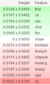
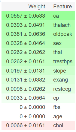
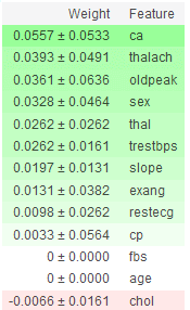
You can see that the two models have very different importance scores for a feature. This can negatively affect the amount of trust you can have in the results.

Nonetheless, we can see that feature like ca, sex, and thal are quite helpful in getting to the correct predictions while age and cp aren’t as crucial for getting to the correct predictions.

Partial Dependence Plots

The partial dependence plot (short PDP or PD plot) shows the marginal effect one or two features have on the predicted outcome of a machine learning model — J. H. Friedman

Concept and Theory

A partial dependence plot gives you information about how a feature affects the model’s predictions. This can help us understand what feature values tend to provide us with higher or lower outputs.

The partial dependence can be calculated easily for categorical features. We get an estimate for each category by forcing all data instances to have the same category. For example, suppose we are interested in how gender affects the chance of having heart disease. In that case, we can first replace all values of the gender column with the value male and average the predictions and then to the same using female as the value.

Calculating partial dependence for regression is more complicated, but Christoph Molnar explains it nicely in his ebook Interpretable Machine Learning. So if you are interested in going deeper into model interpretation, be sure to check it out.

Example and Interpretation

For creating partial dependence plots, we will use the PDPbox library. PDPbox provides us with a few different well-designed plots, including partial dependence plots for a single feature and partial dependence plots for multiple features.

To install PDPbox, we can type:

pip install git+https://github.com/SauceCat/PDPbox.git

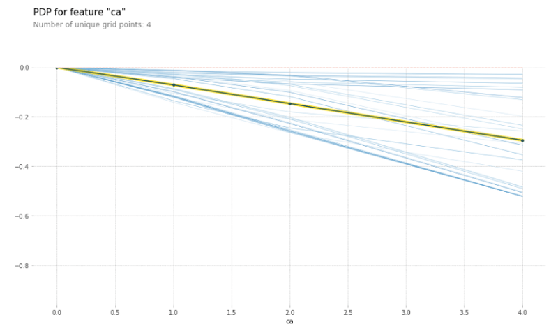
Now we can create a partial dependence plot to analyze the effect of the different genders on the probability of having heart disease using the pdp_isolate and pdp_plot methods.

from pdpbox import pdp, get_dataset, info_plots
pdp_sex = pdp.pdp_isolate(model=lr, dataset=X_test, model_features=feature_names, feature='sex')

pdp.pdp_plot(pdp_sex, 'Gender', plot_lines=True, frac_to_plot=0.5)
plt.show()

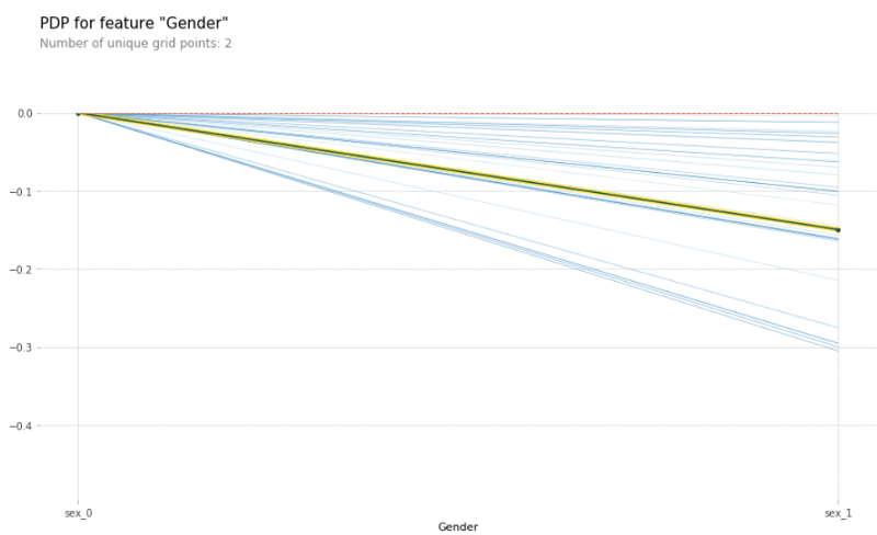
The yellow and black line gives us the average effect on the predictions when changing the gender from sex_0 to sex_1. By only looking at this line, we can see that patients with gender sex_0 are more likely to have heart disease than patients with gender sex_1.

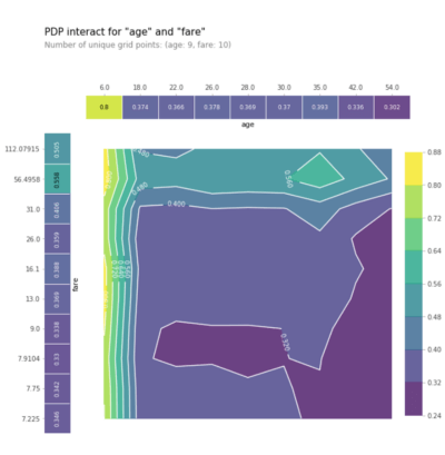
To create a partial dependence plot that shows us the interaction effect of two features on the target, we can use the pdp_interact and  pdp_interact_plot methods.

features_to_plot = ['age', 'sex']
inter1 = pdp.pdp_interact(model=lgb_model, dataset=X_test, model_features=feature_names, features=features_to_plot)

pdp.pdp_interact_plot(pdp_interact_out=inter1, feature_names=features_to_plot, plot_type='contour')
plt.show()

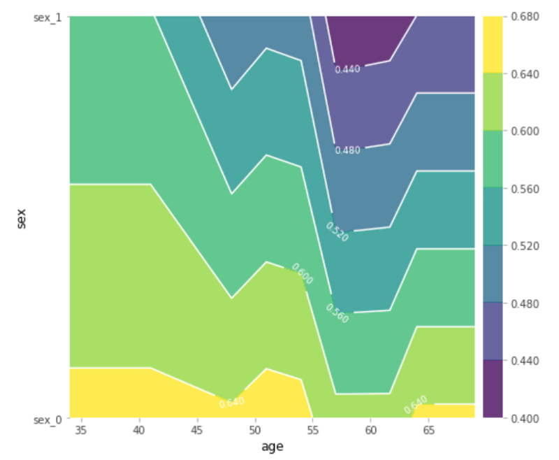
This can help us find interactions between two features or even individual feature values. So, for example, we can see that no matter the value of the gender column, patients aged between 55 and 63 have the lowest probability of having heart disease.

Conclusion

Global model interpretation are techniques that help us to answer questions like how does a model behave in general? What features drive predictions, and what features are completely useless for your cause.

The two most used global model interpretation techniques are feature importance and partial dependence plots.

We can use feature importance to understand how important a model thinks a feature is for making predictions.

Partial dependence plots help us understand how a specific feature value affects predictions. This is extremely useful because it allows you to get interesting insights about specific feature values that can be further analyzed or shared.

What’s next?

In part 3 of this series, we will take a closer look at understanding individual predictions by diving into what local model interpretation is and how two local model interpretation techniques— Lime and Shapely values —  work.

That’s all from this article. If you have any questions or want to chat with me, feel free to contact me via EMAIL or social media.