
As models become more and more complex, it's becoming increasingly important to develop methods for interpreting the model's decisions. I have already covered the topic of model interpretability extensively over the last months, including posts about:
- Introduction to Machine Learning Model Interpretation
- Hands-on Global Model Interpretation
- Local Model Interpretation: An Introduction
This article will cover Captum, a flexible, easy-to-use model interpretability library for PyTorch models, providing state-of-the-art tools for understanding how specific neurons and layers affect predictions.
If you want a more detailed look at Captum, check out its excellent documentation.
Algorithms
Captum includes a large number of different algorithms/methods, which can be categorized into three main groups:
- General Attribution: Evaluates the contribution of each input feature to the output of a model.
- Layer Attribution: Evaluates the contribution of each neuron in a given layer to the output of the model.
- Neuron Attribution: Evaluates the contribution of each input feature on the activation of a particular hidden neuron.
For detailed information about all the available algorithms, check out the algorithm documentation.
General Attribution Techniques
As of now, Captum includes eight algorithms that fall under the General Attribution category. These techniques can be used to evaluate the contribution of input features to the output of a model.
- Integrated Gradients: Represents the integral of gradients with respect to an input along the path of a baseline to the input.
- Gradient SHAP: Is a gradient method to compute SHAP values
- DeepLIFT: A back-propagation based approach to general importance attribution
- DeepLIFT SHAP: A extension of DeepLIFT to approximate SHAP values
- Saliency: Simple approach that returns the gradients of the output with respect to the input
- Input X Gradient: Extention of Saliency that takes the gradients of the output with respect to the input and then multiplies it by the input feature values.
- Guided Back-propagation: Computes the gradient of the target output with respect to the input, but back-propagation of ReLU functions is overridden so that only non-negative gradients are backpropagated. (Only available with the master branch, not with PIP yet)
- Guided GradCAM: computes the element-wise product of guided back-propagation attributions with upsampled (layer) GradCAM attributions (Only available with the master branch, not with PIP yet)
Layer Attribution Techniques
Layer Attribution techniques are great for learning how a particular layer affects the output. Currently, there are five-layer attribution techniques available in Captum:
- Layer Conductance: Combines the neuron activation with the partial derivatives of both the neuron with respect to the input and the output with respect to the neuron to give us a more complete picture of the importance of the neuron.
- Internal Influence: Approximates the integral of gradients with respect to a particular layer along the path from a baseline input to give input.
- Layer Activation: Layer Activation is a simple approach for computing layer attribution, returning the activation of each neuron in the identified layer.
- Layer Gradient X Activation: Like Input X Gradient but for hidden layers.
- GradCAM: Computes the gradients of the target output with respect to the given layer, averages for each output channel (dimension 2 of output), and multiplies the average gradient for each channel by the layer activations. Most often used for convolutional neural networks.
Neuron Attribution Techniques
Neuron attribution methods help you to understand what a particular neuron is doing. They are great when combined with Layer Attribution methods because you can first inspect all the neurons in a layer, and if you don't understand what a particular neuron is doing, you can use a neuron attribution technique.
- Neuron Conductance: Like Layer Conductance but only for a single neuron.
- Neuron Gradient: Neuron gradient is the analog of the saliency method for a particular neuron in a network.
- Neuron Integrated Gradients: Neuron Integrated Gradients approximates the integral of input gradients with respect to a particular neuron along the path from a baseline input to the given input.
- Neuron Guided Backpropagation: Like Guided Backpropagation but for a single neuron.
Captum Example
Using Captum is quite straightforward. You only need a PyTorch model and an example input.
Captum can be installed with the following command:
pip install captum
For demonstration purposes, I will use Captum to analyze the predictions of a pre-trained Resnet18 model.
import torch
import torch.nn.functional as F

from PIL import Image

import os
import json
import numpy as np
from matplotlib.colors import LinearSegmentedColormap

import torchvision
from torchvision import models
from torchvision import transforms

from captum.attr import IntegratedGradients
from captum.attr import GradientShap
from captum.attr import Saliency
from captum.attr import NoiseTunnel
from captum.attr import visualization as viz

torch.manual_seed(0)
np.random.seed(0)

model = models.resnet18(pretrained=True)
model = model.eval()

transform = transforms.Compose([
 transforms.Resize(256),
 transforms.CenterCrop(224),
 transforms.ToTensor()
])

transform_normalize = transforms.Normalize(
     mean=[0.485, 0.456, 0.406],
     std=[0.229, 0.224, 0.225]
 )
The ResNet is trained on the ImageNet data-set. To get more information about the predicted class, we will download the labels.
wget -P <path> https://s3.amazonaws.com/deep-learning-models/image-models/imagenet_class_index.json
labels_path = '<path>/imagenet_class_index.json'
with open(labels_path) as json_data:
    idx_to_labels = json.load(json_data)
Now that we have the model ready, we can download the image we want to use for the analysis.
In my case, I used a picture of a german shepherd.
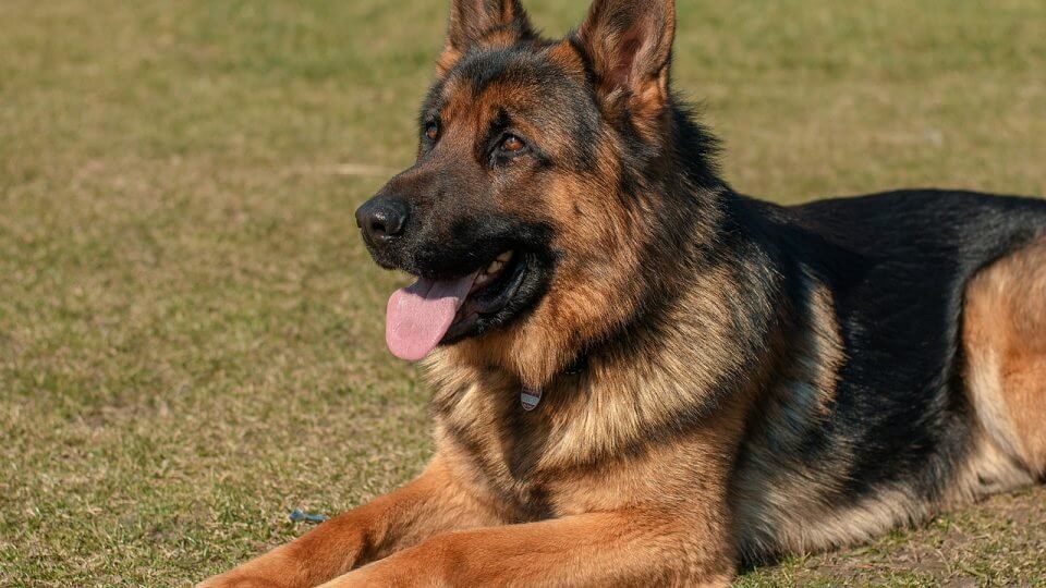
wget -O <path>/dog1.jpg https://www.rover.com/blog/wp-content/uploads/2011/11/german-shepherd-960x540.jpg
img = Image.open('<path>/dog1.jpg')

transformed_img = transform(img)

input = transform_normalize(transformed_img)
input = input.unsqueeze(0)

output = model(input)
output = F.softmax(output, dim=1)
prediction_score, pred_label_idx = torch.topk(output, 1)

pred_label_idx.squeeze_()
predicted_label = idx_to_labels[str(pred_label_idx.item())][1]
print('Predicted:', predicted_label, '(', prediction_score.squeeze().item(), ')')
Predicted: German_shepherd ( 0.9918051958084106 )
The prediction seems correct, but we can't be sure yet that the model learned what a dog looks like. To be sure, we will use General Attribution methods that will help us understand what the model is looking for when making a certain prediction.
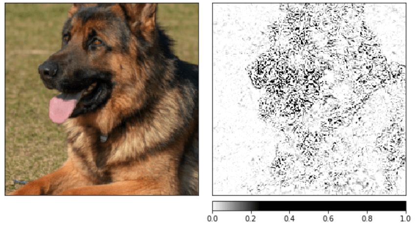
We will start with Integrated Gradients, which represents the integral of gradients with respect to an input along the path of a baseline to the input.
# Create IntegratedGradients object and get attributes
integrated_gradients = IntegratedGradients(model)
attributions_ig = integrated_gradients.attribute(input, target=pred_label_idx, n_steps=200)

# create custom colormap for visualizing the result
default_cmap = LinearSegmentedColormap.from_list('custom blue',
                                                 [(0, '#ffffff'),
                                                  (0.25, '#000000'),
                                                  (1, '#000000')], N=256)


# visualize the results using the visualize_image_attr helper method
_ = viz.visualize_image_attr_multiple(np.transpose(attributions_ig.squeeze().cpu().detach().numpy(), (1,2,0)),
                             np.transpose(transformed_img.squeeze().cpu().detach().numpy(), (1,2,0)),
                             methods=["original_image", "heat_map"],
                             signs=['all', 'positive'],
                             cmap=default_cmap,
                             show_colorbar=True)
The above result gives us a rough idea, but we can get a better image by smoothing the output using a noise tunnel.
noise_tunnel = NoiseTunnel(integrated_gradients)

attributions_ig_nt = noise_tunnel.attribute(input, nt_samples=10, nt_type='smoothgrad_sq', target=pred_label_idx)

_ = viz.visualize_image_attr_multiple(np.transpose(attributions_ig_nt.squeeze().cpu().detach().numpy(), (1,2,0)),
                             np.transpose(transformed_img.squeeze().cpu().detach().numpy(), (1,2,0)),
                             methods=["original_image", "heat_map"],
                             signs=['all', 'positive'],
                             cmap=default_cmap,
                             show_colorbar=True)
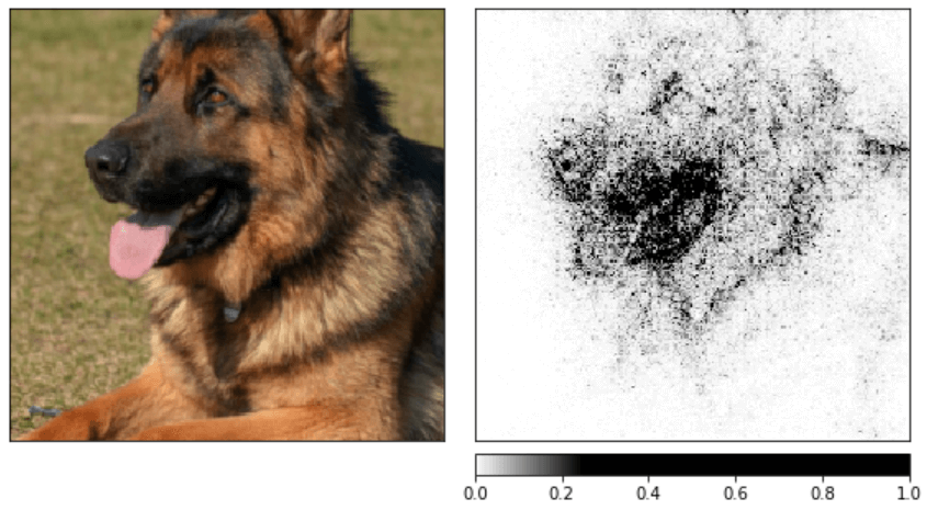
In the above images, we can see that the model heavily focuses on the head of the dog, which is reasonable (at least for me).
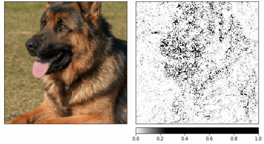
Another great method for gaining insight into the global behavior is GradientShap, a gradient method to compute SHAP values.
gradient_shap = GradientShap(model)

# Defining baseline distribution of images
rand_img_dist = torch.cat([input * 0, input * 255])

attributions_gs = gradient_shap.attribute(input,
                                          n_samples=50,
                                          stdevs=0.0001,
                                          baselines=rand_img_dist,
                                          target=pred_label_idx)
_ = viz.visualize_image_attr_multiple(np.transpose(attributions_gs.squeeze().cpu().detach().numpy(), (1,2,0)),
                             np.transpose(transformed_img.squeeze().cpu().detach().numpy(), (1,2,0)),
                             methods=["original_image", "heat_map"],
                             signs=['all', 'positive'],
                             cmap=default_cmap,
                             show_colorbar=True)
Check out the official documentation for more information about all the available methods.
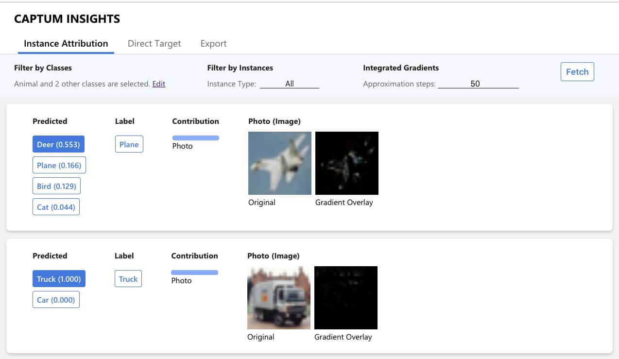
Captum Insights
Even with libraries like Captum, understanding models without proper visualization can still be challenging. Image and text input features can be challenging to understand without these visualizations.
That's why Captum also offers an interpretability visualization widget built on top of it called Captum Insights.
A Captum Insights example can be opened with the following command:
python -m captum.insights.example
Captum Insights also has a Jupyter widget providing the same user interface as the standalone webpage. To install and enable the widget, run:
jupyter nbextension install --py --symlink --sys-prefix captum.insights.widget
jupyter nbextension enable captum.insights.widget --py --sys-prefix
Captum Insights Example
To use Captum Insights, you need to create a data iterator and a baseline function. After creating these two, you need to create an AttributionVisualizer and pass it the model, classes, score function, data iterator, and the baseline function.
Code Example:
from captum.insights import AttributionVisualizer, Batch
from captum.insights.attr_vis.features import ImageFeature

def baseline_func(input):
    return input * 0

def formatted_data_iter():
    dataset = torchvision.datasets.CIFAR10(root='./data', train=False,
                                           download=True, transform=transform)
    dataloader = iter(
        torch.utils.data.DataLoader(dataset, batch_size=4, shuffle=False, num_workers=2)
    )
    while True:
        images, labels = next(dataloader)
        yield Batch(inputs=images, labels=labels)

visualizer = AttributionVisualizer(
    models=[net],
    score_func=lambda o: torch.nn.functional.softmax(o, 1),
    classes=classes,
    features=[
        ImageFeature(
            "Photo",
            baseline_transforms=[baseline_func],
            input_transforms=[transform],
        )
    ],
    dataset=formatted_data_iter(),
)

visualizer.render(debug=False)
You can find a complete example of how to use Captum Insights on my Github.
Conclusion
Captum is a flexible, easy-to-use model interpretability library for PyTorch, providing state-of-the-art tools for understanding how specific neurons and layers affect predictions. Its techniques are split into three categories – General Attribution Techniques, Layer Attribution Techniques, and Neuron Attribution Techniques.
Captum also has an interpretability visualization widget called Captum Insights, allowing users to interpret vision and text models interactively.
That's all from this article. If you have any questions or want to chat with me, feel free to contact me via EMAIL or social media.